| Nonlinear Dynamics Group

Non-smooth Systems

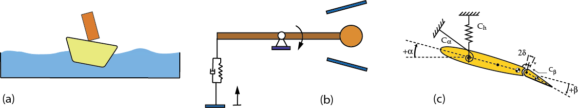
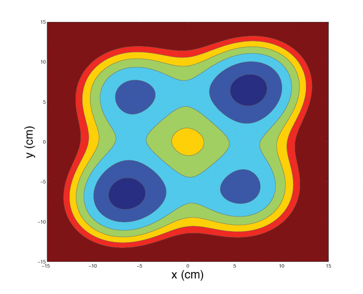
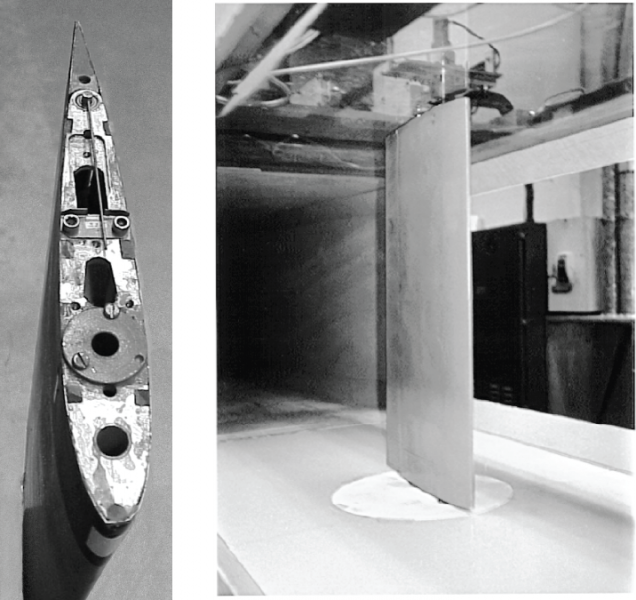
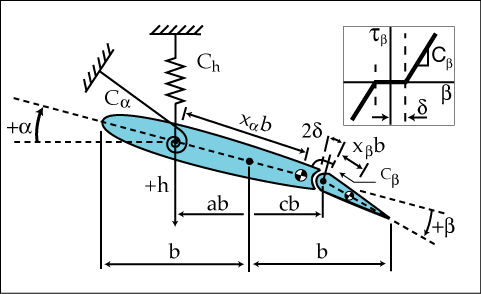
Many dynamical systems (especially mechanical) have discrete non-smooth characteristics. A good number of such systems have been studied in the nonlinear dynamics group here at Duke. One of the motivations for this work is that impacting systems often exhibit limited fatigue life. Non-smooth systems are capable of exhibiting behavior not found in smooth systems, e.g., grazing bifurcations. The systems below have a non-smooth stiffness characteristic:

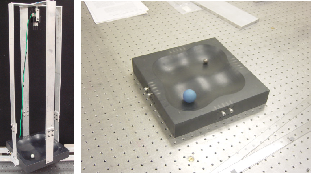
Some other examples are show here:

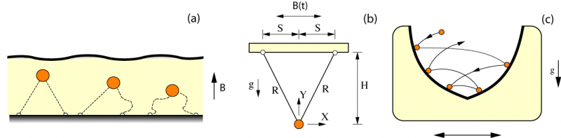
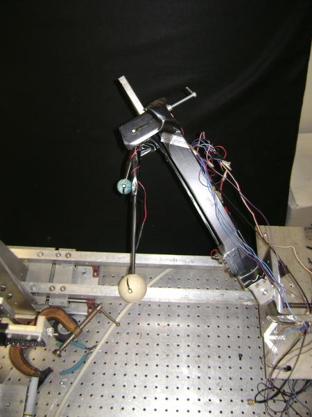
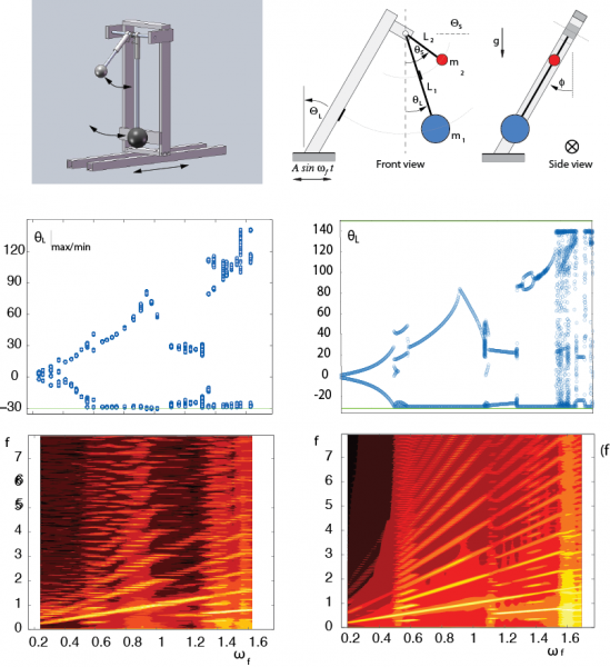
Another example is a double-pendulum impacting system:

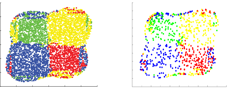
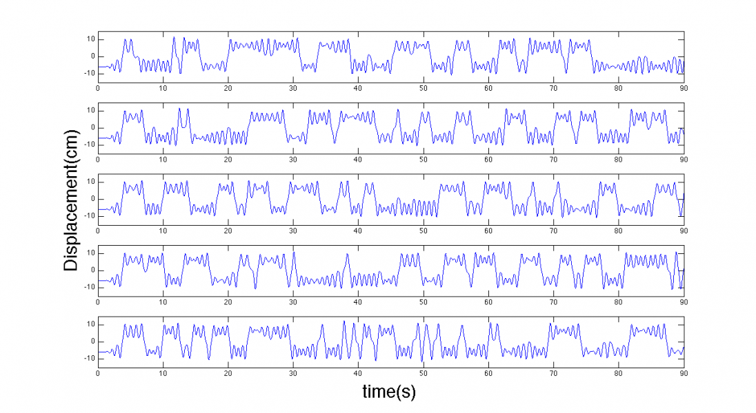
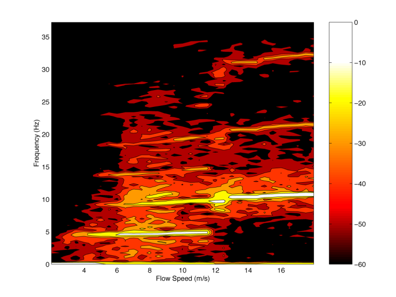
Simulations and experimental data compare very favorably, not just for specific parameter values, but across a broad range (bifurcation diagram and spectragrams). Experimental data on the left, numerical simulation on the right:

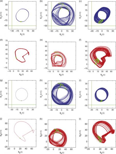
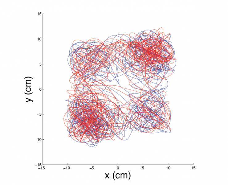
The response at given frequencies can be quite different. For example, below is shown both numerical and experimental data in terms of pseudo-phase projections and Poincaré points (in green) superimposed. (a) - (f) Experimental, (a) and (d) ωf = 1.43, (b) and (e) ωf = 0.58, (c) and (d) ωf=1.51. (g)–(l) Numerical, (g) and (j) ωf=1.415, (h) and (k) ωf=0.5719, (i) and (l) ωf = 1.43.

Ball rolling on a surface

A Rolling Ball System. A conventional paradigm of linear oscillations is the motion of a small ball as it rolls on a parabolic curve with minimal energy dissipation. The unique minimum provides a compelling demonstration of stable equilibrium. If the curve is then shaken at close to the natural frequency of the ball then a large amplitude response occurs due to resonance may occur.

If we take this concept a couple of steps further we can envsion a small ball rolling along a two-dimensional surface, and furthermore, we can design the surface to exhibit various maxima and minima. Now, given some uncertainty in the initial conditions it can be very difficult to predict which long-term behavior (in this case a surface minimum) the ball will eventually end up in (given a little energy dissipation). And if we shake the surface harmonically (say) then chaos is a typical response.

Here is a contour plot of the surface:

and the plots below show initial conditions for the unforced case in which the ball ends up in one of the four minima due to energy dissipation. In these cases the ball is started from rest, i.e., the initial velocity components are zero.

The forced case can produce chaos, first shown as time series and then as phase trajectories:

In the phase projection trajectories overlap (the phase space is 5-dimensional). In both cases (red and blue) the ball is at rest when the forcing is switched on (at the same forcing phase). The inevitable (tiny) difference leads to exponentially diverging behavior - a hallmark of chaos.

Nonlinear Aeroelasticity

The nonlinear behavior and flutter characteristics of an aeroelastic system with control surface freeplay provides a platform for studying some interesting behavior. A low-order, state-space numerical model of the aeroelastic typical section was created which allows for the inclusion of structural freeplay and preload in the control surface degree of freedom. A physical model of the system was also constructed for use in the Duke University low-speed wind tunnel.

One of the most interesting aspects of the behavior of the airfoil is that hysteresis (between types of limit cycle behavior) is present. That is, the type of (flutter) response and the flow speeds at which they occur depends on whether the flow rate is increasing or decreasing. This is nicely captured by the spectrograms shown below.

More details of this research can be found in the paper published in the Royal Society in 2002.

Basins of Attraction

This research considers a global behavior aspect of nonlinear systems - basins of attraction in systems exhibiting bi-stability. Mapping out the final destination of a grid of initial conditions in numerical simulation is quite straightforward. Experimentally, it is much more challenging. However, a system can be subject to a random sequence of disturbances, and making use of a few techniques from nonlinear dyanmics allows a systems dependence on initial conditions to be examined. The following are simply colorful examples, but they can be cross-referenced back to the appropriate publications, listed to the right.

The important point of this research is that (in contrast to linear systems) nonlinear systems are capable of exhibiting long-term recurrent behavior that depends on where the system was started from, and in some cases this dependence on initial conditions is extremely sensitive.

One of the key engineering contexts for basins of attraction is found in the buckling behavior of slender axially-compressed structures: